Optimizing Hospital Placement: A Mathematical Approach to Healthcare Accessibility
Small island nations face unique challenges in healthcare delivery. In Barbados, like many Caribbean islands, hospital facilities adequately serve the population from a medical capacity standpoint. However, geographic barriers, limited transportation options, and concentrated medical facilities in urban centers create significant accessibility gaps for residents in remote parishes. The challenge isn't the quality or capacity of care, but rather the travel burden placed on those living far from existing facilities.
Important: This is a demonstration of optimization techniques using Barbados as an illustrative example. Real healthcare infrastructure planning requires actual population data, road networks, healthcare utilization studies, regulatory constraints, and domain expertise. The parameters and simplifications presented here are for educational purposes to demonstrate the methodology.
Currently, Barbados has one major hospital located at coordinates (13.0956°N, 59.6096°W), serving a population spread across eleven parishes. For this demonstration, we ask: How many additional hospitals might be needed, and where could they be placed to improve accessibility for all residents?
The Optimization Approach
Rather than arbitrarily selecting locations, we demonstrate how mathematical optimization can determine the minimum number of facilities needed to achieve a target coverage level. This approach balances cost efficiency (fewer facilities) with accessibility (adequate coverage).
Geographic Projection: Linearizing the Spherical Surface
A critical first step is transforming geographic coordinates (latitude/longitude on Earth's curved surface) into a flat, linear coordinate system measured in kilometers. This linearization is essential because:
Solver works better in simple geometry space Standard distance calculations, gradient computations, and search algorithms assume a flat geometry. Working directly with latitude/longitude on a sphere introduces nonlinearities that complicate optimization.
The transformation is accurate for small regions. For sufficiently small areas, the Earth's curvature is negligible, and we can treat the surface as locally flat—similar to how a small patch of an orange peel can be pressed flat without distortion.
Maximum effective cap size: This technique works reliably for regions up to approximately 500-800 km in diameter. Beyond this, curvature effects become significant and more sophisticated projections (e.g., UTM, Lambert Conformal Conic) are needed.
Why it works for Barbados: The island measures only ~34 km × 23 km, well within the acceptable range. At this scale, the equirectangular projection introduces negligible error, making distance calculations effectively identical to those on a true spherical surface.
The projection uses these transformations:
centerLon, centerLat = centroid of Barbados boundary
x (km) = (lon - centerLon) × earthRadius × cos(centerLat) × π/180
y (km) = (lat - centerLat) × earthRadius × π/180
This converts degrees to kilometers while accounting for latitude-dependent longitude scaling.
Model Variables
Our optimization model considers each potential hospital location as having two coordinates in a projected kilometer space:
v = [x₀, y₀, x₁, y₁, x₂, y₂, ..., x₁₄, y₁₄]
This creates 15 potential facility slots (30 dimensions total). The solver can eliminate facilities by positioning them outside Barbados' boundary, and only facilities inside the boundary are considered.
Fixed Facilities: Accounting for Existing Infrastructure
The existing hospital at (-7.1, -10.3) km in projected space is treated as a parameter, not a variable.
This means:
- The existing hospital always contributes to coverage
- The solver doesn't waste iterations trying to relocate it
- New facilities are optimized around the existing infrastructure
- Total facilities = 1 fixed + N variable optimized locations
Objective Function
The model minimizes a composite objective that balances facility cost against coverage shortfall:
minimize: activeFacilities × cost + coverageShortfall × penalty

where:
  activeFacilities = number of facilities inside Barbados boundary
  coverageShortfall = max(0, targetCoverage - actualCoverage)
  cost = 1.0 (per facility)
  penalty = 1000.0 (per % below target)
Coverage is calculated using an exponential decay model with a 5 km service radius, representing a reasonable travel distance for hospital access in a small island context. The high penalty (1000×) ensures the model prioritizes meeting the 95% coverage target before minimizing facility count.
Target Coverage
We target the ten parish centers (excluding St. Michael) as representative population centers:
- Christ Church (-59.528861, 13.091183)
- St. Philip (-59.467710, 13.135766)
- St. John (-59.506853, 13.173657)
- St. George (-59.544516, 13.145151)
- St. Thomas (-59.587743, 13.181953)
- St. Joseph (-59.544599, 13.206338)
- St. James (-59.622557, 13.192131)
- St. Andrew (-59.580215, 13.242278)
- St. Peter (-59.612472, 13.259414)
- St. Lucy (-59.618642, 13.304817)
Coverage Calculation
For each parish center, we calculate coverage from all facilities:
- Calculate distance to all facilities (fixed + active variable)
- Compute coverage:
coverage = exp(-distance / 5 km) - Take maximum coverage from any facility
- Parish is "covered" if
coverage ≥ coverageThreshold (0.3)
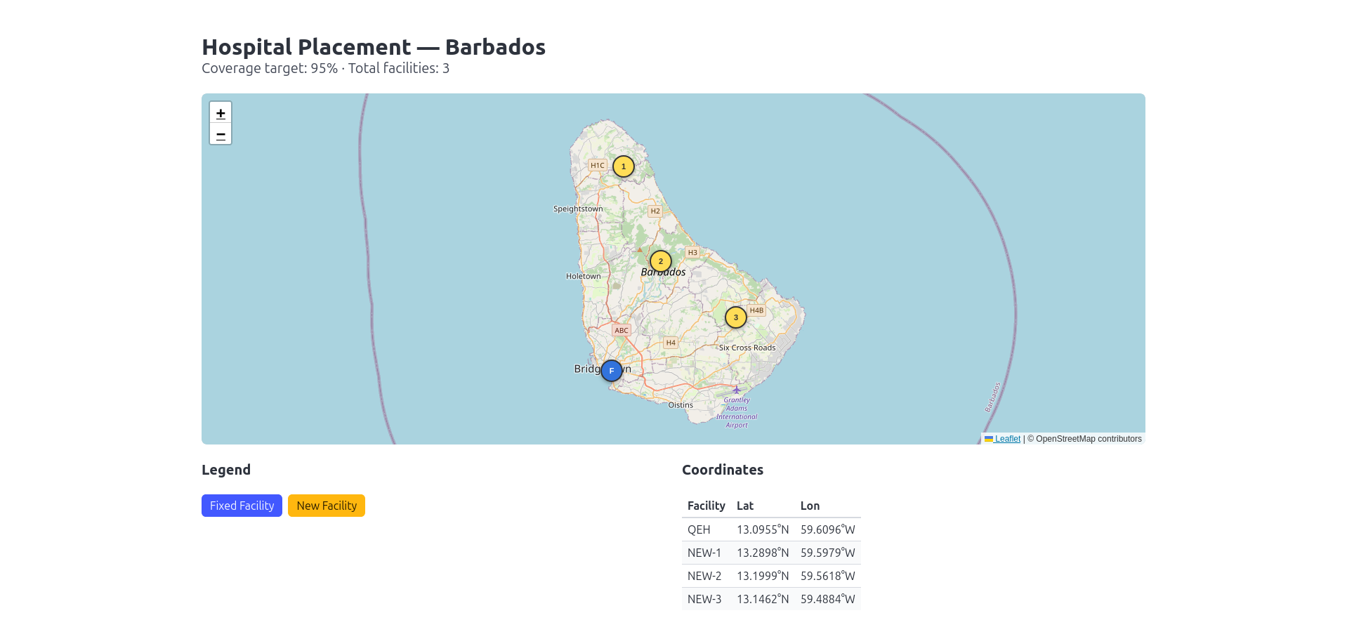
Results: Optimal Hospital Placement
Solution Summary
The optimization solver will determine the minimum number of additional hospitals needed to complement the existing facility and achieve 95% coverage of all parish centers with a 5 km service radius.
═══════════════════════════════════════════════════════
FACILITY PLACEMENT RESULTS - BARBADOS
═══════════════════════════════════════════════════════

FIXED FACILITIES (existing, always deployed):
Facility   Projected (km)       Geographic
───────────────────────────────────────────────────────
FIXED-1    (-7.1, -10.3)         13.0955°N, 59.6096°W

NEW FACILITIES (optimized placement):
Facility   Projected (km)       Geographic
───────────────────────────────────────────────────────
NEW-1      (-5.8, 11.3)         13.2898°N, 59.5979°W
NEW-2      (-1.9, 1.3)         13.1999°N, 59.5618°W
NEW-3      (6.0, -4.7)         13.1462°N, 59.4884°W

═══════════════════════════════════════════════════════
SUMMARY
═══════════════════════════════════════════════════════
Fixed facilities: 1
New facilities needed: 3
Total facilities: 4
Objective value: 4.00
Coverage target: 95%
Optimization Parameters
serviceRadius = 5.0             // Service radius per hospital
coverageThreshold = 0.3         // Minimum coverage level
targetCoverage = 0.95           // 95% parish coverage goal
facilityCost = 1.0              // Cost per facility
shortfallPenalty = 1000.0       // Penalty for missing coverage
Running the Optimization
The optimization is executed using a custom non-linear mesh-based solver with the following parameters:
let meshParams =
    { Channels = 256
      MaxIterations = 4096
      Order = SortOrder.Minimum
      Tolerance = 0.001
      Bounds =
        [ "X0",  [ -20.0; 25.0 ]; "Y0",  [ -25.0; 20.0 ]
          "X1",  [ -20.0; 25.0 ]; "Y1",  [ -25.0; 20.0 ]
          "X2",  [ -20.0; 25.0 ]; "Y2",  [ -25.0; 20.0 ]
          "X3",  [ -20.0; 25.0 ]; "Y3",  [ -25.0; 20.0 ]
          "X4",  [ -20.0; 25.0 ]; "Y4",  [ -25.0; 20.0 ]
          "X5",  [ -20.0; 25.0 ]; "Y5",  [ -25.0; 20.0 ]
          "X6",  [ -20.0; 25.0 ]; "Y6",  [ -25.0; 20.0 ]
          "X7",  [ -20.0; 25.0 ]; "Y7",  [ -25.0; 20.0 ]
          "X8",  [ -20.0; 25.0 ]; "Y8",  [ -25.0; 20.0 ]
          "X9",  [ -20.0; 25.0 ]; "Y9",  [ -25.0; 20.0 ]
          "X10", [ -20.0; 25.0 ]; "Y10", [ -25.0; 20.0 ]
          "X11", [ -20.0; 25.0 ]; "Y11", [ -25.0; 20.0 ]
          "X12", [ -20.0; 25.0 ]; "Y12", [ -25.0; 20.0 ]
          "X13", [ -20.0; 25.0 ]; "Y13", [ -25.0; 20.0 ] ]
    }

let response = Cruiser.solveMesh meshParams facilityPlacement client
Notice that only fourteen bounds are used. This is due to the existing facility which is considered in the evaluation expression. We only need to optimize for the 28 remaining points but have the 2 points from existing facilty still involved for the distance calculations.
Bounds: The search space extends beyond Barbados' physical boundaries (approximately -10 to 16 km in X, -15 to 15 km in Y). This is intentional as the bounds must be wide enough to allow the solver to "deactivate" facilities by pushing them outside the boundary. Facilities placed outside Barbados don't contribute to coverage and aren't counted in the facility cost, effectively removing them from the solution.
Channels & Iterations: 256 parallel evaluation channels with up to 4096 iterations provide thorough exploration of the solution space for this 28-dimensional problem (14 facilities × 2 coordinates).
// Submit optimization job
submit()

// Fetch results (use correlation ID from submit)
// fetchResult "your-correlation-id-here"
Model Limitations
While this optimization demonstrates a powerful methodology, real-world healthcare infrastructure planning requires addressing several simplifications made in this example:
Geographic Simplifications
Euclidean distance vs road networks: This model uses straight-line distance. Actual travel times depend on road quality, traffic, terrain, and available transportation modes.
Uniform terrain assumption: Mountains, water bodies, and other geographic features create accessibility barriers not captured in simple distance metrics.
Population & Demand
Equal parish weighting: Parishes have vastly different populations. Real planning must weight coverage by actual population distribution.
No demand modeling: Hospital utilization depends on demographics, health conditions, emergency vs routine care, and existing healthcare facilities beyond major hospitals.
Missing facility types: This focuses on hospitals but ignores clinics, urgent care centers, specialty facilities, and telehealth infrastructure.
Healthcare-Specific Factors
Service differentiation: Emergency services require different proximity than routine care. Specialized services (cardiac, oncology) have different coverage requirements.
Capacity constraints: Real hospitals have limited beds, staff, and equipment. Location optimization must be paired with capacity planning.
Regulatory & political realities: Land availability, zoning, construction costs, staffing constraints, and political considerations all influence feasibility.
Model Parameters
Arbitrary service radius: The 5 km radius is illustrative. Real planning requires analyzing actual patient travel patterns and acceptable response times.
Coverage threshold: The exponential decay model with threshold 0.3 is a mathematical convenience, not a validated healthcare accessibility metric.
Bottom line: This is a methodological demonstration. Actual healthcare infrastructure decisions require collaboration between optimization specialists, healthcare planners, government agencies, community stakeholders, and domain experts with access to real data.
Conclusion
This example demonstrates how mathematical optimization can provide a data-driven framework for infrastructure planning decisions. While the model includes necessary simplifications, it illustrates a powerful approach to balancing competing objectives: minimizing facility costs while maximizing population accessibility.
This pattern could be adapted for many infrastructure placement problems. The same formulation approach applies to:
Transmission poles for electrical grid expansion Cell towers for telecommunications coverage Service stations for fuel/EV charging networks Fire stations for emergency response Schools for educational access Water treatment facilities for utility infrastructure
Any facility placement problem with coverage requirements and cost constraints can benefit from this approach.
Let's Talk
Interested in applying these optimization techniques to real-world problems? Have a facility placement challenge with actual data? I'm happy to discuss how these methods can be adapted and extended with proper domain expertise, real datasets, and practical constraints. Reach out via the contact details on this site.