Buggy route planning using Integer Programming
A search-and-rescue UGV picks its way across rough terrain. A planetary rover queues its next move while a satellite transmits fresh imagery. Both share a planning problem: pick the next move while the world is still updating.
We build the planner core for that pattern. A region-discretized grid over continuous terrain. The goal is to reach the target in the shortest amount of time and adapt as the world changes. We leverage the F# DSL for OrTools, and execute it on the remote solver service armada.
Why discretize
LP and MILP solve in milliseconds and can leverage the existing toolset developed over the years. The grid simplifies the problem to the point where we can increase or decrease cell resolution as needed, which affects solve speed and path smoothness. Lower resolution produces harsh turns; light post-processing smooths them. Picking the right resolution matters, but this post skips that.
The resolution also determines how many items to track. For an embedded system on the move, faster world updates mean fresher inputs and better plans. For our purposes, some external service publishes free cells and obstacles on each time instance (tick) — drone, satellite, SLAM stack, sensor fusion. The planner does not care which. Bad inputs make bad plans; that is a perception problem, not a planner problem.
Pre-processing
A cell is a list of integer coordinates. Two-element for the 2D buggy here; three or more for vertical or full volumetric planning. The same pre-processing code works at any dimension because none of it hardcodes a length.
type Cell = int list   // [i; j] in 2D, [i; j; k] in 3D, ...

type GridSpec = {
    Dimensions: int list   // [width; height] in 2D
    CellSize: float
}
Three helpers do the geometry. allCells enumerates the Cartesian product of dimensions. neighbors produces the 3^N − 1 candidates around a cell. edgeCost counts how many coordinates differ between two cells, multiplying cell size by √differing — cardinal moves (one differing coordinate) cost the cell size, 2D diagonals cost √2 ×, 3D corner moves cost √3 ×, and so on:
let allCells (dimensions: int list) : Cell seq =
    let extend acc dim =
        seq {
            for partial in acc do
                for i in 0 .. dim - 1 do
                    yield partial @ [i]
        }
    List.fold extend (seq { yield [] }) dimensions

let neighbors (cell: Cell) : Cell seq =
    let extend acc i =
        seq {
            for partial in acc do
                for di in -1 .. 1 do
                    yield partial @ [i + di]
        }
    List.fold extend (seq { yield [] }) cell
    |> Seq.filter (fun candidate -> candidate <> cell)

let edgeCost (cellSize: float) (a: Cell) (b: Cell) =
    let differing =
        List.zip a b
        |> List.filter (fun (x, y) -> x <> y)
        |> List.length
    cellSize * sqrt (float differing)
Free cells and edges fall out of these. Diagonal moves get one extra guard so the buggy can't clip an obstacle corner — for any move differing in 2+ dimensions, the orthogonal side cells must also be free:
let inBounds (grid: GridSpec) (cell: Cell) =
    List.zip cell grid.Dimensions
    |> List.forall (fun (c, d) -> c >= 0 && c < d)

let freeCells (grid: GridSpec) (obstacles: Set<Cell>) : Set<Cell> =
    allCells grid.Dimensions
    |> Seq.filter (fun cell -> not (obstacles.Contains cell))
    |> Set.ofSeq

let isMoveAllowed (free: Set<Cell>) (a: Cell) (b: Cell) =
    let differingDims =
        List.zip a b
        |> List.mapi (fun i (ai, bi) -> if ai <> bi then Some i else None)
        |> List.choose id
    if List.length differingDims < 2 then true
    else
        differingDims
        |> List.forall (fun d ->
            let side =
                a |> List.mapi (fun i v ->
                    if i = d then v
                    elif List.contains i differingDims then b.[i]
                    else v)
            free.Contains side)

let edges (grid: GridSpec) (free: Set<Cell>) : (Cell * Cell * float) list =
    [
        for cell in free do
            for neighbor in neighbors cell do
                if inBounds grid neighbor
                   && free.Contains neighbor
                   && isMoveAllowed free cell neighbor then
                    yield (cell, neighbor, edgeCost grid.CellSize cell neighbor)
    ]
Roughly 4,500 directed edges on a 24 × 24 grid with light obstacle coverage.
The IP
Shortest path in graph terms — given a directed graph G = (V, E) with non-negative edge costs cij, a source s, and a sink t, find the path from s to t that minimizes the sum of edge costs along it.
For the buggy: V is the set of free cells, E is the set of N-connected directed edges between free cells, cij is the traversal cost of edge (i, j), s is the buggy's current cell, and t is the goal.
Encoded as an integer program — one binary variable xij per directed edge, set to 1 if the edge is used and 0 otherwise. Flow conservation at every node. Minimize total cost:
minimize    ∑_{(i,j) ∈ E}  c_{ij} · x_{ij}

subject to  ∑_{(k,j) ∈ E} x_{kj}  −  ∑_{(i,k) ∈ E} x_{ik}  =  b_k    ∀ k ∈ V

            x_{ij} ∈ {0, 1}                                          ∀ (i,j) ∈ E

where       b_s = +1     (source — net outflow of one unit)
            b_t = −1     (sink   — net inflow of one unit)
            b_k =  0     for k ∈ V \ {s, t}
The flow-conservation row for node k says: outflow minus inflow equals supply. The source supplies one unit, the sink absorbs one unit, every other node passes flow through unchanged. The unique x assignment that satisfies this with binary variables is exactly the indicator of an s –> t path.
open Operations.Research.Types
open Operations.Research.Models

let edgeName (tail: Cell) (head: Cell) =
    let render = List.map string >> String.concat "_"
    sprintf "x_%s__%s" (render tail) (render head)

let buildModel
    (cells: Cell list)
    (graphEdges: (Cell * Cell * float) list)
    (source: Cell) (goal: Cell) =

    // x_ij in [0, 1]. TU lets us solve as an LP and read off integers.
    let variables =
        graphEdges
        |> List.map (fun (tail, head, _) ->
            Variable.real (edgeName tail head) 0.0 1.0)

    let edgesAndVars = List.zip graphEdges variables

    // Pre-index by tail and head — each conservation row becomes a Map
    // lookup instead of a full edge scan.
    let outByCell =
        edgesAndVars
        |> List.groupBy (fun ((tail, _, _), _) -> tail)
        |> Map.ofList

    let inByCell =
        edgesAndVars
        |> List.groupBy (fun ((_, head, _), _) -> head)
        |> Map.ofList

    let conservation cell =
        let outSum =
            Map.tryFind cell outByCell
            |> Option.defaultValue []
            |> List.map snd
            |> LinearExpression.sum
        let inSum =
            Map.tryFind cell inByCell
            |> Option.defaultValue []
            |> List.map snd
            |> LinearExpression.sum
        let netFlow = outSum + (-1) * inSum
        let supply =
            if cell = source then  1.0
            elif cell = goal  then -1.0
            else                    0.0
        netFlow === supply

    let objective =
        edgesAndVars
        |> List.map (fun ((_, _, cost), variable) -> cost * variable)
        |> LinearExpression.sum

    Model.empty
    |> DecisionVars variables
    |> Goal Minimize
    |> Objective objective
    |> Constraints (cells |> List.map conservation)
Variable.real with bounds [0, 1] is correct — total unimodularity (next section) guarantees the LP relaxation lands on integers, and that is cheaper than declaring booleans.
The total-unimodularity footnote
The LP relaxation of this IP returns integers automatically — no branch-and-bound, no Variable.boolean. The property that buys this is total unimodularity (TU): when the constraint matrix A is TU and the right-hand side b is integer, every vertex of the feasible polytope has integer coordinates, so simplex lands on an integer point by construction. A matrix is TU when every square submatrix has determinant in {−1, 0, +1}.
The flow-conservation matrix of any directed graph is TU. Rows index nodes, columns index edges; each column has exactly one +1 (the head) and one −1 (the tail), and zeros elsewhere. That is a textbook TU pattern. Combined with integer right-hand sides ({+1, 0, −1}), the LP relaxation of the shortest-path IP is the IP.
The payoff — GoogleLinear (a continuous LP solver) returns binary values from result.Variables. For 24 × 24, both LP and MIP return in milliseconds; the difference is irrelevant. The property is fragile, though — any side constraint with arbitrary coefficients (a deadline, an energy budget, a required-waypoint set) breaks TU and forces real branch-and-bound.
The replan loop
The outer loop owns the tick counter and the buggy's current cell. At each tick: pull obstacles from the sensor model, recompute the free set and edges, build and submit the model, normalize the result, record a PathFrame, advance one cell along the planned path. Repeat until the buggy reaches the goal or the loop hits a max.
Tick length and maxTicks together set the planner's real-time budget. Exceed it and the loop terminates with the buggy short of the goal — the deadline beat the planner.
type FrameStatus =
    | Optimal of cost: float
    | Feasible of cost: float
    | Infeasible of message: string

type PathFrame = {
    Tick: int
    BuggyCell: Cell
    Goal: Cell
    Obstacles: Set<Cell>
    PlannedPath: Cell list
    Status: FrameStatus
    SolveTimeMs: float
}

let runReplan
    (grid: GridSpec)
    (client: Cruiser)
    (obstaclesAt: int -> Set<Cell>)
    (source: Cell) (goal: Cell)
    (maxTicks: int) : PathFrame list =

    Seq.unfold (fun (tick, current) ->
        if tick > maxTicks || current = goal then None
        else
            let frame = solveAt grid client obstaclesAt tick current goal
            let nextCell =
                match frame.PlannedPath with
                | _ :: stepCell :: _ -> stepCell
                | _                  -> current   // already at goal or no path
            Some (frame, (tick + 1, nextCell))
    ) (0, source)
    |> Seq.toList
The model builder stays pure on cell data — same inputs, same model. The loop attaches metadata and dispatches to the solver. This separation matters when you want to replay a frame or swap the solver backend without touching the planner.
Run #1 — static field
24 × 24 grid. Source at (1, 1), goal at (22, 22). Four obstacle features: a vertical wall, a rectangular cluster, a long horizontal blocker near the top, a small cluster near the goal. The replan loop runs to completion and produces a single HTML page with one subplot per tick.
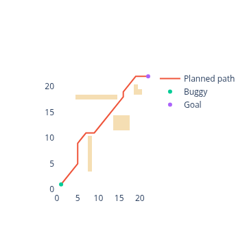
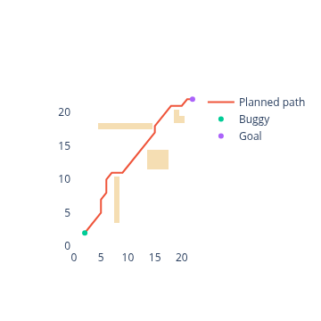
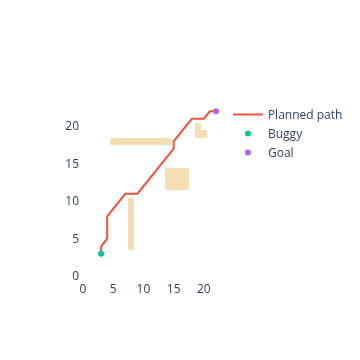
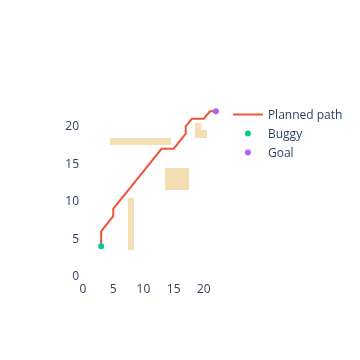
Run #2 — obstacle injected mid-run
Same starting field. At tick 5, a new rock cluster lands across the planned corridor — a moving truck, a competitor vehicle, a sand drift. The replan reflects it the moment the new free set propagates.
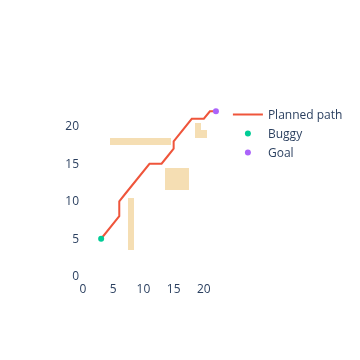
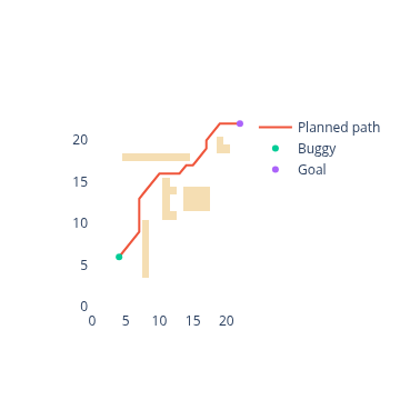
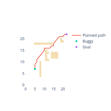
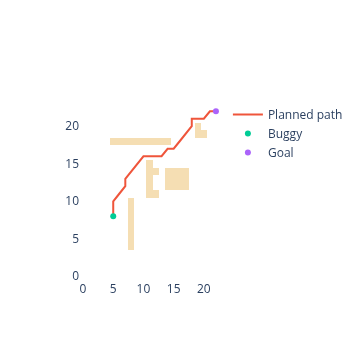
The server's solve stays in single-digit milliseconds; the per-tick budget is dominated by the round trip to the solver. Every step must finish inside the tick window.
Performance caveats
=== Scenario A: static field ===
  ticks: 27
  reached goal: true
  solve time ms: median 36.0, Q1 34.0, Q3 37.0

=== Scenario B: injection at tick 5 ===
  ticks: 29
  reached goal: true
  solve time ms: median 33.0, Q1 31.0, Q3 35.0
Thirty-something milliseconds per tick, dominated by the network round trip. An s –> t shortest path on 576 cells is not what a MILP solver finds hard — most of that budget is in the request and response, not the search. Three ideas to bring it down:
Reuse the previous plan. A replan does not start from nothing — the buggy already has a path it was about to follow. Truncate that path from the current cell to the nearest unblocked cell on the remaining course, and build the next model around that as a warm start (fixed prefix, free suffix). Most ticks change nothing about the obstacle field, so most of the plan is still valid; only the bend around the new obstacle needs solving. Smaller model means smaller payload and smaller server-side solve — both halves of the budget come down.
Co-locate the solver. Drop the remote solver round trip — call in-process. Eliminates serialization, network, and queue. The bulk of the per-tick budget should go with it.
Coarser cells. Doubling cell size quarters the variable count. Fine when terrain features are larger than the new cell, otherwise obstacles get clipped into low-resolution blobs.
For a buggy ticking once a second, none of this matters as a demo. For a buggy ticking ten times a second, all three start to matter much, much more.