Districts Without Redistricting
Every week this year brought another redistricting headline. Texas redrew its congressional map mid-decade to net five new seats; California answered with about five of its own; more states followed. By now an increasing number of House seats have been redrawn outside the normal census cycle — through special sessions, legislator walkouts, and lawsuits. Both sides burned months and millions to move a handful of seats. There must be a better use of that time.
Why the current method is doomed
The root problem is population. We draw districts to hold equal headcounts, so every census ( and every convenient mid-decade excuse) reopens the map. Population is the one input guaranteed to change, which guarantees the fight recurs. So I asked a different question: what if the map never moved?
Two countries pointed the way. Sweden barely draws districts at all — it inherits its counties as multi-member seats and repairs proportionality nationally. Canada does the hard part well: an independent commission picks a target size, then draws each province's ridings around that target within a target band. I grafted the two. Take Canada's target-and-band discipline, but instead of cutting fresh lines, keep the county borders already on the map. Group whole counties into contiguous clusters near a fixed target. Population never enters, so population can never trigger a redraw. The House seats 435 members, so the map must produce 435 groups. And that count, spread across the country's land, fixes each group near a target size.
That was the idea. Getting a computer to do it took three tries, and the first two were wrong in instructive ways.
Attempt one: the integer program
My instinct was optimisation. Set a binary variable for every county-and-group pair — county i is a member of group j — open as few groups as possible, keep each under an area cap, and let a solver minimise the group count. Clean on paper.
Two things went wrong. First, contiguity: a group has to be one connected blob, and an assignment solver will happily scatter a group across a state to hit a nicer number. I spent most of my time here — first with a heavy network-flow encoding, then a lighter "attachment" rule (every county must border a fellow group member) plus a repair pass. That part came good.
The second problem I misread for a long time: The model would not scale. Nevada, seventeen counties, solved in a fraction of a second. Oregon, thirty-six, took a full minute and still couldn't prove it was done. California never returned at all. I kept blaming the contiguity math. I was wrong as the flaw was the word minimise. Asking for the fewest possible groups makes the solver prove no smaller number exists — an exhaustive search over a combinatorial space — and that proof is what strangled it. I hadn't yet noticed I was solving a much harder problem than I needed to.
Attempt two: the greedy algorithm
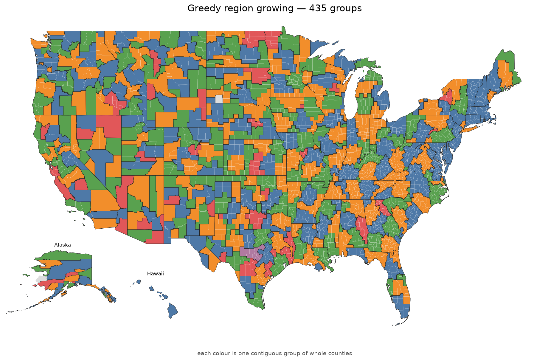
While the solver churned, I wrote a crude fallback: start from the largest county, absorb its neighbours until the group hits the area cap, then start again with the next-largest county still unclaimed. Because it only ever swallows a bordering county, every group is connected for free. It drew the whole country — 3,142 counties — in under a tenth of a second.
def grow_state_into_groups(counties):
    # largest county first, then swallow bordering counties until the cap is hit
    largest_first = sorted(counties, key=lambda name: (-counties[name]["area"], name))
    assigned, groups = set(), []
    for start in largest_first:
        if start in assigned:
            continue
        members, total = [start], counties[start]["area"]
        assigned.add(start)
        while True:
            # only ever consider a county that already borders the group
            candidate = next(
                (nb for m in members for nb in neighbours[m]
                 if nb not in assigned
                 and total + counties[nb]["area"] <= GROUP_AREA_LIMIT),
                None)
            if candidate is None:
                break
            members.append(candidate)
            assigned.add(candidate)
            total += counties[candidate]["area"]
        groups.append(members)
    return groups
Fast and simple, but greedy and blind: it strands outliers. A county whose neighbours are all taken becomes a lonely one-county group, and that happens to roughly a quarter of all groups, clustered in the sparse West. A usable draft, not a good map.
Attempt three: the constraint program
Then the thing I should have seen at the start: this is a combinatorial problem, not an optimisation. I already knew how many groups I wanted. There was never anything to minimise. I only had to find some partition that fit the rules.
That one change rewrites everything. Fix the group count up front, drop the objective, and hand the same constraints — one group per county, seeds anchoring each group, the area band, the attachment rule — to a constraint solver (CP-SAT) instead of an optimiser. Now it isn't proving a number is smallest; it's just searching for a valid arrangement, and stops at the first one it finds.
Here is the whole model. Fix the seeds, cap the area, demand attachment, and ask for a partition:
model = cp_model.CpModel()
group = [model.NewIntVar(0, groups_wanted - 1, f"g{i}") for i in range(n)]

# each seed anchors its own group
for seed, g in seed_group.items():
    model.Add(group[seed] == g)

in_group = {}
for i in range(n):
    for g in range(groups_wanted):
        flag = model.NewBoolVar(f"in_{i}_{g}")
        model.Add(group[i] == g).OnlyEnforceIf(flag)
        model.Add(group[i] != g).OnlyEnforceIf(flag.Not())
        in_group[i, g] = flag

# the area cap: no group may exceed it
for g in range(groups_wanted):
    model.Add(sum(area[i] * in_group[i, g] for i in range(n)) <= group_cap[g])

# attachment: every non-seed county must share its group with a neighbour
for i in range(n):
    if i in seed_group:
        continue
    shared = []
    for j in adjacency[i]:
        same = model.NewBoolVar(f"s_{i}_{j}")
        model.Add(group[i] == group[j]).OnlyEnforceIf(same)
        model.Add(group[i] != group[j]).OnlyEnforceIf(same.Not())
        shared.append(same)
    if shared:
        model.Add(sum(shared) >= 1)
The last constraint asks each county to share its group with at least one neighbour. That sounds like contiguity. It is not. A group can satisfy it while sitting in three separate clumps, each clump perfectly attached to itself. Attachment forbids a lone island; it does not forbid an archipelago. I did not appreciate that for a long time.
So a repair pass is needed where it walks out from each seed to see what is genuinely reachable, and reassigns anything cut off to a bordering group.
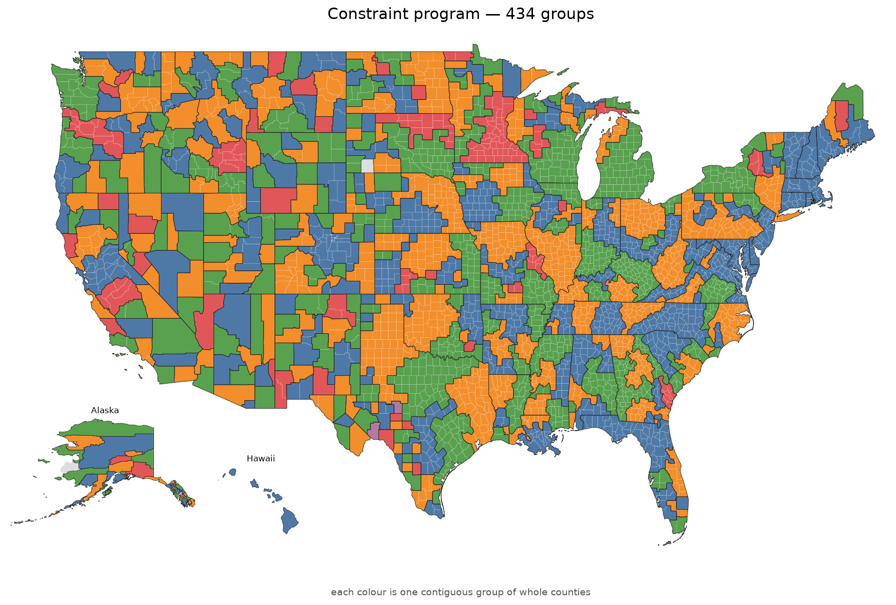
The difference is night and day: California solves in 0.3 seconds; Texas — 254 counties, the state that was hopeless — in 2.8. The entire nation resolves in about 12 seconds, 434 groups, every state feasible (a band that widens only where geography demands it handles the awkward ones), and after the repair pass, every group but a single island county hangs together as one piece. Where a state won't fit the band, the solver returns the near-miss and flags the stragglers — the one-county leftovers a human then places, breaking the cap where a real special case demands it. A solver proposes; a person finishes.
Results
Run across all 3,142 counties, the two working methods land here:
| Groups | Single-county groups | Median group | Largest group | Time | |
|---|---|---|---|---|---|
| Greedy | 435 | 107 | 4 counties | 45 counties | 0.08s |
| Constraint program | 434 | 179 | 2 counties | 75 counties | ~14s |
Both maps come out contiguous bar a single island county — but they get there very differently, and that difference is the story. The greedy is contiguous by construction: it only ever adds a county that already borders the group, so it cannot produce a broken one. The constraint program is not: its groups arrive in fragments and the repair pass stitches them back together, which works, but bills the area cap for it. And surprisingly, the greedy draws the more balanced map. Its regions are larger while the constraint program leaves nearly twice as many single county "groups". Wherever a single county already exceeds the area target (most of the sparse West), that county is its own group no matter what draws it, and the greedy only hides more of them by packing to a slightly higher limit. A two-sided band that forces groups to fill makes several states infeasible outright.
Four states, up close
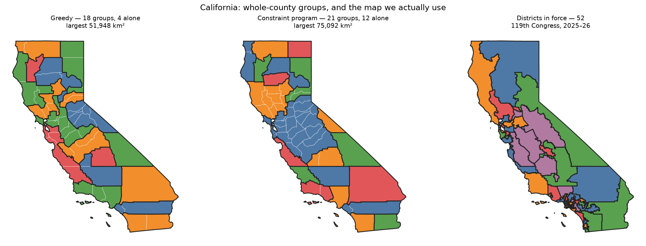
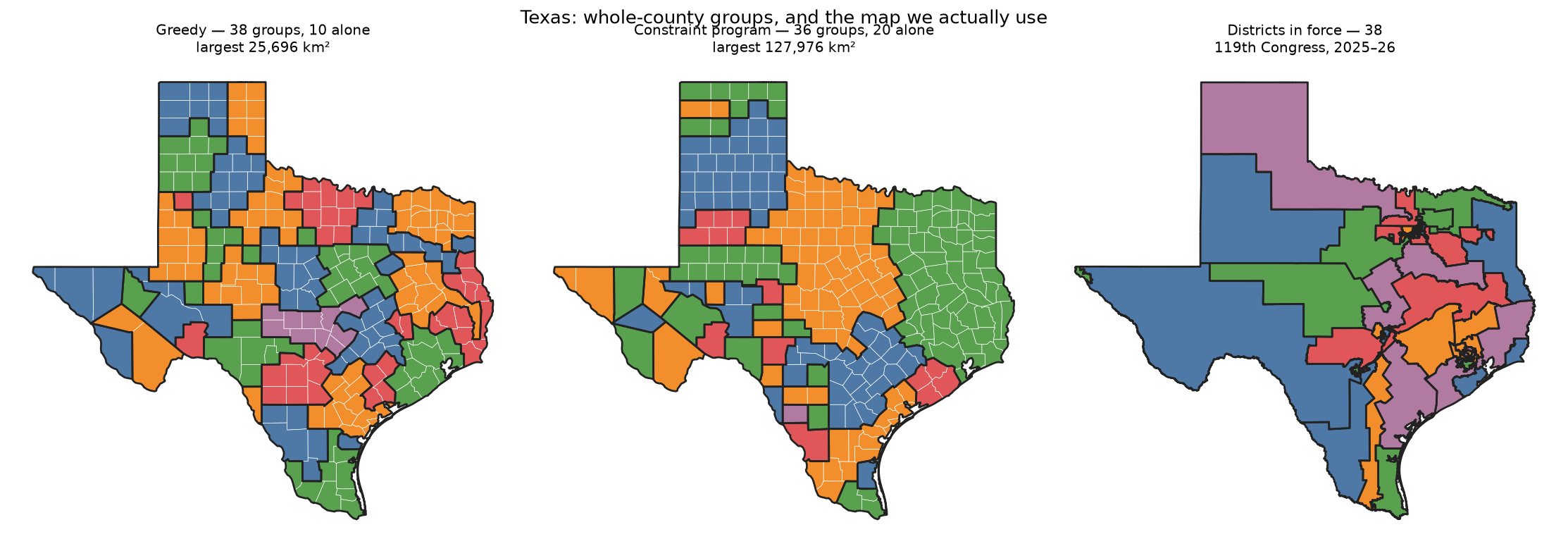
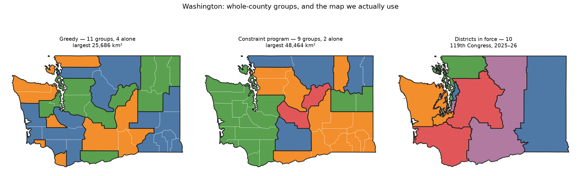
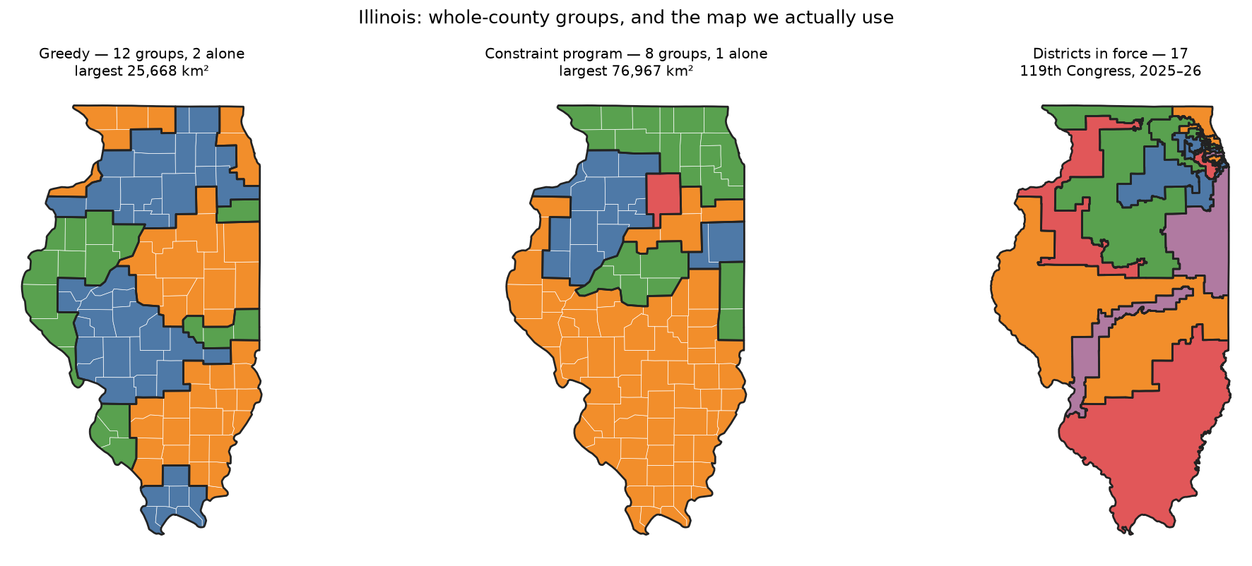
The national totals hide what the two methods do differently, so here are four states drawn three ways — greedy, the constraint program, and the districts in use today.
Two things jump out.
The first is that the constraint program's groups sprawl, and drawing them is what showed me why. Texas is the worst case: its largest group covers 127,976 km², nearly seven times the target (where the greedy's largest is 25,696). Illinois runs 76,967 km² against greedy's 25,668 km²; Washington, 48,464 km² against greedy's 25,686 km². Illinois, in particular, one group swallows most of the state's southern region, where intuitively it should be two or three.
That sprawl is the repair pass at work. The constraint program's attachment rule keeps every county touching a group-mate, but it does not force a group to hang together as one piece, so the raw output arrives with groups in scattered fragments. The flip repair then merges those fragments back into whole regions — which is what the map needs — and in doing so drags the group areas far past the cap. The count settling near 435 is a by-product of that merging, not its purpose. Contiguity gets bought at the expense of maintaining the area cap.
The greedy has no such bill, and there is a neat way to see it: run the same flip repair over the greedy's output and nothing happens at all. Identical groups, identical areas, identical stragglers, in every state. The repair only ever fires on a county cut off from its seed, and the greedy — which never adds a county unless it borders the group already — never produces one. The repair is a treatment for a condition only found in the constraint formulation.
That does not make the greedy optimal since it strands 107 counties nationally, and its balance is a rule of thumb, not a proof. But it is reasonable in context where the constraint program is not.
The second is Washington, the one state that runs against the national grain. There the constraint program strands 2 counties to the greedy's 4, and covers the state in 9 groups where the greedy needs 11 — the greedy leaves Clark, Thurston and Wahkiakum orphaned in the southwest corner. Everywhere else in this sample the greedy strands fewer: 4 against 12 in California, 10 against 20 in Texas, 2 against 1 in Illinois. So the national finding holds — the greedy draws the tidier map — but not uniformly, and Washington is the honest counterexample.
| Counties | Greedy groups / alone | Constraint groups / alone | Greedy largest | Constraint largest | Districts today | |
|---|---|---|---|---|---|---|
| California | 58 | 18 / 4 | 21 / 12 | 51,948 km² | 54,927 km² | 52 |
| Texas | 254 | 38 / 10 | 36 / 20 | 25,696 km² | 127,976 km² | 38 |
| Washington | 39 | 11 / 4 | 9 / 2 | 25,686 km² | 48,464 km² | 10 |
| Illinois | 102 | 12 / 2 | 8 / 1 | 25,668 km² | 76,967 km² | 17 |
The third panel in each figure is the point of the whole exercise. Set the county groups beside the districts actually in force and the difference in kind is obvious: the groups follow borders that already exist and that nobody drew for advantage, while the districts wander across counties in shapes that only make sense once you know what they were drawn to achieve.
A district drawn to hit a headcount can be reopened whenever the headcount moves, and a shape with no constraint beyond arithmetic can be bent toward any end its author likes. A group of whole counties has fewer places to hide: the borders are inherited, the rule is public, and the result is dull enough that there is little to litigate. Counties are also numerous and varied enough that grouping them still yields a mix of people. Enough population variation exists inside each group to make a real contest without any of it depending on a line drawn to a purpose.
So the honest verdict is not the one I expected to write. The constraint program is scalable and it is genuinely useful for what it reports — a hard band it either meets or flags, and an explicit list of the special cases a human must settle. But it does not enforce the one property this whole problem is about, and it leans on a post-process to paper over that. The greedy enforces it for free, runs the nation in 0.08 seconds, and draws the better map.
One more difference tilts toward the greedy (and it matters for anything public): it is deterministic. The same counties always yield the same map, because the rule is fixed — largest county first, neighbours in sorted order. The constraint program only promises a feasible map that fits; ask it twice and you can get two different valid partitions. In redistricting, reproducibility isn't a nicety, it's required. The difference between a map anyone can re-derive and audit and one you have to take on trust. You can pin the constraint program down — a fixed search seed, or tie-breaking constraints — but every such constraint nudges it back toward the very optimisation it just escaped.
Landing exactly on 435
The constraint run returns 434 because the sparse states can't produce their land-share of groups (Alaska tops out at one per borough). Treat the gap as routine and close it deliberately.
Short of 435 — spend the spare seats where they mean the most. Extend the map to the U.S. territories, which the land-only pass ignores. Or hand the leftover seats back to the states by population, splitting the groups sitting on the largest headcounts first. Population, banished from the method to keep the map stable, returns only here, at the margin where it nudges toward real representation without ever being able to trigger a full redraw.
Over 435 — merge. Fuse the thinnest marginal groups with a neighbour until the count drops to 435.
Either way, the adjustment is a handful of moves a person makes in an afternoon, not a year-long statewide redraw.
Where it works, and where it doesn't
It works because the map is frozen by construction: no census reopens it, no official discovers a fresh reason to redraw. It runs on public data anyone can audit — borders and areas, no voter files, no partisan lean — and finishes in seconds what commissions and courts drag out for a year.
It works poorly because land is blunt. It ignores where people actually live, so an empty county counts like a crowded one. And freezing the map freezes its unfairness (especially if there is little migration). This method draws a 90% usable map and a human still finishes the last stretch (transparently of course).
None of that makes it worse than what we run today. The current system spends a year and a fortune to produce maps drawn to be partisan. This spends seconds to produce maps drawn to be dull.......and dull (and cheap) beats contested, costly, and (possibly) rigged.
Sources
- Redistricting ahead of the 2026 elections — Ballotpedia, state-by-state tracker
- Mid-Decade Congressional Redistricting: Key Issues — Congressional Research Service
- What's happening with gerrymandering in the United States — Harvard Kennedy School, May 2026
- An Emerging Trend: Mid-Decade Redistricting — Voting Rights Lab, May 2026
- All About Redistricting — Loyola Law School, litigation tracker
- Changing the Maps — National Conference of State Legislatures
- 2025–26 Mid-Decade Redistricting Map — Cook Political Report
The district boundaries
The congressional district map above is the 119th Congress (2025–26) — the districts in force as I write. The boundaries come from the UCLA cdmaps project:
- Repository: github.com/JeffreyBLewis/congressional-district-boundaries (MIT licensed)
- Project page: cdmaps.polisci.ucla.edu
The date matters more than usual here. The collection covers every district in use from 1789 through 2025, built under NSF grant SBE-SES-0241647 between 2009 and 2013 and augmented since with boundaries published by the Census Bureau and state agencies.
The 120th Congress will not use the map above: California and Texas have already been redrawn, while Missouri, North Carolina, Utah and Ohio sit in litigation whose outcome is unresolved. Any picture of "the current districts" is a photograph with a timestamp, and that is the whole problem this post is about. The county groups, by contrast, would still be the county groups.
Geographical data
Everything else runs on public files anyone can re-download and check.
- Counties, land area, centroids — 2019 county file via the evangambit/JsonOfCounties.
- County adjacency — github.com/btskinner/spatial
- County boundaries (maps only) — github.com/plotly/datasets county GeoJSON, keyed by FIPS.